The Brilliance of Norman Lloyd Johnson's Unbounded System

[Dilettante]

Oi!

I've noticed that the forum has plenty of threads for reacting to content (X, Rumble, and YouTube) and relating over discussion topics, but I was surprised to find only a few threads devoted to original and creative personal pursuits. I'd like to see more of this kind of stuff, whether it's mathematics or science or mysticism.

So, I'd like to share with you my favorite statistical distribution, some cool numerical tools in the R language, and hopefully work all the way up to a terse yet powerful machine learning algorithm that I find really, really interesting.

Let's begin with the distribution, my absolute favorite.

Norman Lloyd Johnson was a student of Egon Pearson, who in turn was the son of Karl Pearson, who studied under Francis Galton, and if you follow the line of teachers way up you'll find Isaac Newton! This is the real heart of the academic spirit, having an excellent mentor. Anyways, in his 1949 paper entitled "Systems of Frequency Curves Generated by Methods of Translation," Johnson details what he calls the Sᵤ distribution ("unbounded system").

A sample of parameterized probability density functions (PDFs) from the Sᵤ can be seen here:



Like the Gaussian (Normal) distribution, Johnson's Sᵤ is unimodal, meaning it has one hump. The normal distribution controls for location on the X-axis (mean) and the scale or width of the tails (standard deviation). In addition to these parameters, the Sᵤ also controls for skewness (is one tail heavier than the other?) and kurtosis (is the peak flat or pointy?). In the Sᵤ, these parameters are called gamma, delta, xi, and lambda. It's important to remember there is no one-to-one correspondence between the parameters and the moments using this distribution.

A collection of functions for use in the R language is as follows, with the same usage as the distribution functions found in the standard library:

djohnson <- function(x, gamma = 0, delta = 1, xi = 0, lambda = 1) {
    z <- (x - xi) / lambda
    scale <- delta / (lambda * sqrt(2 * pi))
    shape <- 1 / sqrt(1 + z ^ 2)
    tail <- exp(-0.5 * (gamma + delta * asinh(z)) ^ 2)
    scale * shape * tail
}

pjohnson <- function(q, gamma = 0, delta = 1, xi = 0, lambda = 1) {
    pnorm(gamma + delta * asinh((q - xi) / lambda))
}

qjohnson <- function(p, gamma = 0, delta = 1, xi = 0, lambda = 1) {
    xi + lambda * sinh((qnorm(p) - gamma) / delta)
}

rjohnson <- function(n, gamma = 0, delta = 1, xi = 0, lambda = 1) {
    xi + lambda * sinh((qnorm(runif(n)) - gamma) / delta)
}

That's a good start for now.

Okay, so what's so great about this distribution? It works for negative, zero, and positive numbers. It controls for central tendency, dispersion, asymmetry, and kurtosis. This basically covers most unimodal organic data! I'm not joking! It's not perfect, but it's really, really good.

I use this distribution in finance to model equity returns, it's way better than log-normal. Leagues better. We'll figure out how to parameterize this distribution later.

Ciao!

[Dilettante]

Okay. Before we get too far into this project, we have to learn about numerical optimization. This is a huge topic, in part born out of a much forgotten but brilliant interdisciplinary field called operations research. If I ever got another degree, this would be a strong candidate.

We're going to keep it very simple, so we'll only really cover a hill climbing algorithm and the Nelder-Mead method, and mostly from a practical standpoint, not a technical one.

I think a good place to start and retain relevance to the end goal would be first to use a hill climbing algorithm to parameterize a normal distribution one moment at a time, then use the Nelder-Mead method to parameterize both moments of the normal distribution at once, and end with the parameterization of Johnson's Su. Let's dive in!

We need some data to work with, so in the R language we can use the default dataset `cars` for some easy to understand X-Y data:



We have two variables, `speed` and `dist` referring to how far the stopping distance of the car is at a given speed. We can see in the marginal density plots that `speed` is distributed fairly normally, although with a much flatter peak than a Gaussian, and that `dist` is distributed asymmetrically with respect to its tails.

Let's work with `dist` for now, try out both a normal and Johnson's Su on it. First, let's figure out how to use the `optimize` function in R. This is not a hill climbing algorithm (Apologies! We could make one if you're really curious), it's a more sophisticated search function, but it only operates on a single variable. We give it a loss function to minimize and a range in which to search:

x <- cars$dist

optimize(f = function(mu) sum((x - mu)^2),
         interval = range(x))

# > optimize(function(mu) sum((x - mu)^2), range(x))
# $minimum
# [1] 42.98

# $objective
# [1] 32538.98

# > mean(x)
# [1] 42.98

What's going on here? We define our X variable as `dist` from the `cars` dataset. We define our loss function as the sum of squared residuals between all values in X against a candidate mean (`mu`). We tell the search to proceed within the range of our X values. The result, which is found commented out, is the minimized `objective` and its corresponding candidate called the `minimum`. As we can verify, this minimum is the same as the mean!

Let's subtract the mean and then find the standard deviation:

x1 <- cars$dist - 42.98

optimize(f = function(sigma) sum((sqrt(mean(x1^2)) - sigma)^2),
         interval = range(abs(x1)))

# > optimize(f = function(sigma) sum((sqrt(mean(x1^2)) - sigma)^2),
# +          interval = range(abs(x1)))
# $minimum
# [1] 25.51038

# $objective
# [1] 0

We should note that this standard deviation doesn't use Bessel's correction like most standard functions. We found that our `dist` function has a mean of 42.98 and a raw standard deviation of 25.51. How would we do both of these at the same time?

Instead of the `optimize` function, we can use the `optim` function, which optimizes multiple variables at once. I like to do this iteratively, first getting a rough parameterization using quantiles, then a closer fit using something like a K-S test or negative log-likelihood:

x <- cars$dist

qqtad <- function(p) {
    sum(abs(p - seq(0, 1, length.out = length(p))))
}

one <- optim(par = c(0, 1),
             fn = function(ms) qqtad(pnorm(x, ms[1], ms[2])[order(x)]))

two <- optim(par = one$par,
             fn = function(ms) -sum(log(dnorm(x, ms[1], ms[2]))))

# > one
# $par
# [1] 40.18027 25.05558

# $value
# [1] 1.594726

# > two
# $par
# [1] 42.98534 25.51202

# $value
# [1] 232.9012

The first fit is like a baby version of the K-S test. The second fit, we're using MLE estimation instead of a K-S test, but both could work. Notice we found the mean and the standard deviation at the same time! This is absolutely necessary for working with the Johnson Su. Unlike the normal, where the parameters can be found one at a time, because the parameters are simply the moments, this will not be the case in the Johnson Su.

I'll leave it at that for now and come back later to tackle the parameterization of the Johnson Su. There's plenty of meat in this post, but if you can understand and be comfortable working with optimizers, a whole new world opens up! They are a seriously powerful tool in your toolbox for solving problems.

[Dilettante]

Let's knock this out. Fitting the Johnson Su to our `dist` variable.

The good news? It's the exact same process as the above, we'll get a rough estimate of the parameters and then refine it:

x <- cars$dist

one <- optim(par = c(0, 1, 0, 1),
             fn = function(gdxl) {
                 p <- pjohnson(x, gdxl[1], gdxl[2], gdxl[3], gdxl[4])
                 qqtad(p[order(x)])
             })

two <- optim(par = one$par,
             fn = function(gdxl) {
                 d <- djohnson(x, gdxl[1], gdxl[2], gdxl[3], gdxl[4])
                 -sum(log(d))
             })

Really nothing crazy, other than we have four parameters for the Johnson Su instead of the two for the Gaussian. It's the exact same process for any distribution actually. Go crazy with this! Find a cool distribution on Wikipedia with the formula for the CDF and PDF? You can parameterize it!

Alright, let's see how it's looking using a density plot:



Notice how much closer the Johnson Su is to the raw kernel density estimate compared to the normal? That's what it's all about.

Next up, we'll perform joint normalization between two variables, then things start to get interesting.

[Dilettante]

Slight detour, just for fun.

Want to know what a linear model is? At least for two variables, it's actually really simple and plenty interesting (I still chew on how simple yet unintuitive this is).

x <- cars$speed
y <- cars$dist

n <- length(x)

x_bar <- sum(x) / n
y_bar <- sum(y) / n

x_dev <- x - x_bar
y_dev <- y - y_bar

m <- sum(x_dev * y_dev) / sum(x_dev^2)
b <- y_bar - m * x_bar

y_hat <- m * x + b

Or, in text form:

• The predicted value of Y is found by adding the Y-intercept to the product of the slope and each X value.
• The Y-intercept is calculated by subtracting the product of the slope and the mean of X from the mean of Y.
• The slope is determined by dividing the covariance between X and Y by the variance of X.
• The covariance is the sum of the products of the deviations of each X and Y value from their means, while the variance of X is the sum of the squared deviations of each X value from its mean.
• The means of X and Y are the averages of their respective datasets.

And we end up with the nice red line:



There you have it. A simple linear regression operating under ordinary least squares. I'll get to joint normalization as promised, but I wanted to show you the vanilla approach first.

[Dilettante]

Alright, joint normalization it is. But what is it?

It's simply the process of applying normalization to 2 or more variables at the same time. Why do that? To linearize a model prediction! For two variables, it's not too dissimilar from normalizing each variable independently, modeling the result, and transforming the result back to the original scale for the dependent variable. For three or more variables, it has a more pronounced effect.

To do this for our `speed` and `dist` variables, it looks like this:

x <- cars$speed
y <- cars$dist

opt <- optim(par = c(0, 1, 0, 1, 0, 1, 0, 1),
             fn = function(prm) {
                 xp <- pjohnson(x, prm[1], prm[2], prm[3], prm[4])
                 yp <- pjohnson(y, prm[5], prm[6], prm[7], prm[8])
                 m <- lm(qnorm(yj) ~ qnorm(xj))
                 sum(log(cosh(m$residuals)))
             })

We are simply normalizing X and Y at the same time, mapping it to the normal distribution for each variable, then modeling those normals, and finally scoring the fit by a loss function on the residuals.

If you are familiar with loss functions, you'll notice that I use log-cosh loss above, which I believe is the "best of both worlds" as it is robust when the function is far away from the minimum, but precise as it gets close. Robust like MAE yet precise like squared:



From the parameters, we can model Y in transformed space, then reverse the process on the results back to the original variable space.

prm <- opt$par
xp <- pjohnson(x, prm[1], prm[2], prm[3], prm[4])
yp <- pjohnson(y, prm[5], prm[6], prm[7], prm[8])

m <- lm(qnorm(yj) ~ qnorm(xj))
zp <- pnorm(m$fitted.values)

z <- qjohnson(zj, prm[5], prm[6], prm[7], prm[8])

And we're left with a prediction like this!



Notice how the curve fits just a bit better than a straight line? We did that!

What's the point of this? It's not so different than modeling the log-Y by log-X, which can be addressed manually... Well, that's exactly the point. By joint normalization, we can use optimizers to transform our variable space automatically and minimize loss on residuals, no human needed!

We're one step away from a machine learning algorithm, believe it or not.

[Dilettante]

We're close to finishing, but we have to address another little tidbit first. How does the Johnson Su actually work? Let's take a look at its CDF:

pjohnson <- function(q, gamma = 0, delta = 1, xi = 0, lambda = 1) {
    pnorm(gamma + delta * asinh((q - xi) / lambda))
}

Essentially, although the operations are a little different, we have two linear transformations of location and scale happening here. In the original variable space, xi locates and lambda scales. Then, in asinh space, gamma locates and delta scales. Then, this transformed variable is fed into the Gaussian CDF, so Johnson has cleverly "recycled" all that math here.

It's not 100% correct to say that xi and lambda are vanilla location and scale normalization, as lambda is applied after location in the original space, whereas gamma and delta function as a more traditional normalization pair. This is important because we have xi locate X before we scale it using lambda into asinh space. The easiest way to describe asinh space is as log-like but extending into negative numbers and including zero.

How does that work?

asinh <- function(x) ln(x + sqrt(x^2 + 1))

This function is so clever, I love it. By squaring X, adding one, taking that square root, and adding it back onto X, we ensure that our domain is bounded above zero for a range from negative infinity to infinity. When we take the log of this domain, we have a log-like function that works into a negative range!



There's something magical about the inverse hyperbolic functions. Notice we have already used cosh in a loss function, so the hyperbolic functions themselves are pretty neat as well. I'm not going to pretend I understand their complexity, but as someone who thinks in curves and not formula, it was a boon to find such functions!

So, yes, the real magic of the Johnson Su can be found in the clever use of the inverse hyperbolic sine (asinh) function, which feeds into the Gaussian CDF to create its own CDF. I like thinking of asinh like a French curve, you can find the perfect curve on some little portion of it and extend that into your variable space.

We're almost there! Now that we know about the magic of asinh, we're ready to make our machine learning regression algorithm.

[Dilettante]

It's time to finish it. First, we'll need some helper functions:

sum_log_cosh <- function(m) {
    sum(log(cosh(m$residuals)))
}

gasinh <- function(x, xi = 0, lambda = 1) {
    asinh((x - xi) / lambda)
}

gsinh <- function(x, xi = 0, lambda = 1) {
    sinh(x) * lambda + xi
}

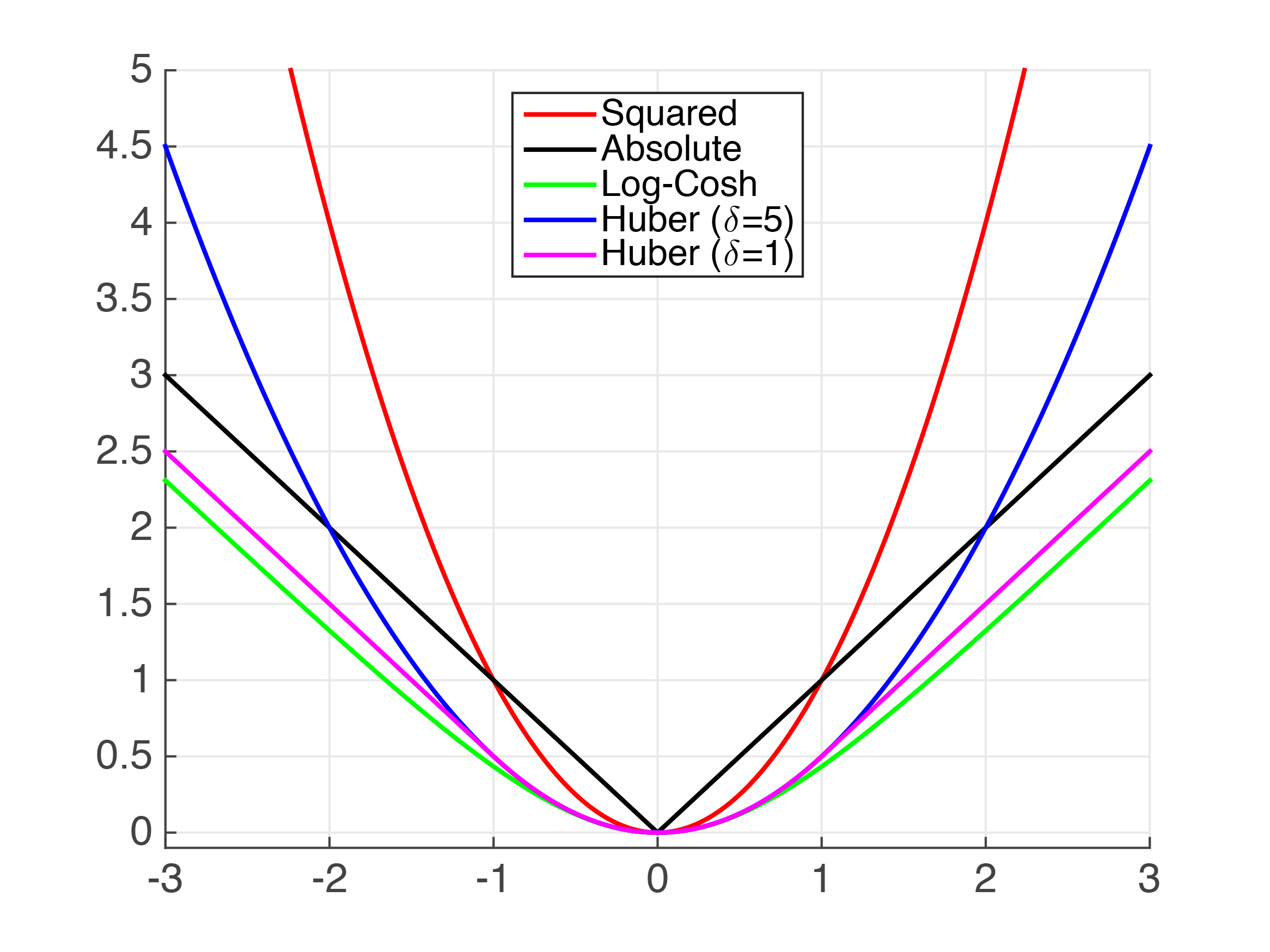
Above, we have the log-cosh loss function from earlier, then a generalized form of the asinh function and its inverse, sinh.

Why don't we have gamma and delta anymore? Well, this is because when we use a linear model, each variable has a coefficient associated with it that acts exactly like delta does. There is an additional coefficient (the Y-intercept) that essentially replaces all of the gammas into a single summation. So both of these parameters are redundant within the context of a linear model.

Now, onto the big kahuna:

lm.gat <- function(formula, data = NULL,
                   loss = sum_log_cosh,
                   iterations = 1, penalty = 1e-9,
                   verbose = FALSE) {

    as.df <- as.data.frame
    use.gasinh <- function(i, df, prm) {
        gasinh(df[, i], prm[2 * (i - 1) + 1], prm[2 * (i - 1) + 2])
    }

    env <- if (is.null(data)) environment(formula) else as.environment(data)
    sub <- as.df(sapply(all.vars(formula), get, envir = env))

    n <- ncol(sub)
    prm <- rep(c(0, 1), n)

    evaluate <- function(prm) {
        mut <- setNames(as.df(sapply(1:n, use.gasinh, sub, prm)), names(sub))

        tryCatch({
            m <- lm(formula, mut)
            cost <- penalty * mean(prm ^ 2)
            loss(m) + cost
        }, error = function(e) {
            Inf
        })
    }

    for (k in 1:iterations) {
        opt <- optim(prm, evaluate)
        prm <- opt$par
        if (verbose) {
            message("Loss: ", format(opt$value, scientific = TRUE))
        }
    }

    prm <- opt$par
    mut <- setNames(as.df(sapply(1:n, use.gasinh, sub, prm)), names(sub))
    m <- lm(formula, mut)

    detransform <- function(y) gsinh(y, prm[1], prm[2])

    list(detransform = detransform,
         par = prm,
         fit = m,
         opt = opt,
         df.sub = sub,
         df.mut = mut,
         z = detransform(m$fitted.values))
}

It's not exactly easy to explain this function - which isn't perfect, by the way. It will only well on continuous random variables and the transformation is applied to all variables in the model, so it's not very customizable. Essentially, for all variables including the response, we have an associated pair of parameters which transforms that variable in asinh space. These parameters are wiggled around by the optimizer, minimizing loss on the residuals. What's neat is that it can optimize interactive models as well.

Let me demonstrate. Let's say we are using the built-in `mtcars` dataset. We will try to predict quarter-mile time (`qsec`) by horsepower, miles per gallon, and weight (`hp`, `mpg`, `wt`) in a full interactive model:

summary(lm(qsec ~ hp * mpg * wt, mtcars))

# Call:
# lm(formula = qsec ~ hp * mpg * wt, data = mtcars)

# Residuals:
#     Min      1Q  Median      3Q     Max
# -1.5219 -0.5882 -0.0978  0.4013  3.1959 

# Coefficients:
#               Estimate Std. Error t value Pr(>|t|)
# (Intercept) 14.0426771 10.9005197   1.288    0.210
# hp           0.0017784  0.0590665   0.030    0.976
# mpg          0.0249053  0.3921269   0.064    0.950
# wt           0.2427188  3.4981471   0.069    0.945
# hp:mpg      -0.0005924  0.0026322  -0.225    0.824
# hp:wt        0.0016601  0.0179826   0.092    0.927
# mpg:wt       0.1050975  0.1451373   0.724    0.476
# hp:mpg:wt   -0.0003813  0.0008658  -0.440    0.664

# Residual standard error: 1.102 on 24 degrees of freedom
# Multiple R-squared:  0.7055,    Adjusted R-squared:  0.6196 
# F-statistic: 8.215 on 7 and 24 DF,  p-value: 4.052e-05

This is a simple approach using the original variable space, nothing is transformed. Notice the p-value is highly significant, but we only have an R-squared value of 70.5%, meaning that that amount of variation in the response variable is explained by our model. Furthermore, none of our coefficients are significant on their own, meaning this model is over-parameterized.

Let's try with our auto-transforming model:

summary(lm.gat(qsec ~ hp * mpg * wt, mtcars, iterations = 5)$fit)

# Call:
# stats::lm(formula = formula, data = mut)

# Residuals:
#        Min         1Q     Median         3Q        Max
# -0.0025768 -0.0006795  0.0001064  0.0006047  0.0023484

# Coefficients:
#               Estimate Std. Error  t value Pr(>|t|)
# (Intercept)  1.986e+00  7.537e-04 2635.538  < 2e-16 ***
# hp           7.993e-04  1.277e-04    6.259 1.81e-06 ***
# mpg         -8.981e-04  4.055e-04   -2.215 0.036518 *
# wt          -5.751e-03  5.441e-04  -10.568 1.65e-10 ***
# hp:mpg       2.700e-04  5.836e-05    4.627 0.000107 ***
# hp:wt       -2.916e-04  1.005e-04   -2.902 0.007821 **
# mpg:wt      -1.725e-03  2.280e-04   -7.566 8.34e-08 ***
# hp:mpg:wt   -1.658e-04  2.609e-05   -6.354 1.43e-06 ***
# ---
# Signif. codes:  0 '***' 0.001 '**' 0.01 '*' 0.05 '.' 0.1 ' ' 1

# Residual standard error: 0.001372 on 24 degrees of freedom
# Multiple R-squared:  0.9142,    Adjusted R-squared:  0.8891
# F-statistic: 36.52 on 7 and 24 DF,  p-value: 2.732e-11

The R-squared value shot up to 91.4%, so we've captured that much more variation in the response variable! Now all of the coefficients are significant, and the overall model p-value is extremely significant.

So what's going on? The optimizer seeks to linearize all of these relationships, all at once. Since log-cosh is a very robust yet precise loss function, this works pretty well.

We have a very small, understandable, machine learning program here. It works automatically with no need for a human to go in and determine the best transformation for each variable. It's robust because it uses a generalized unimodal distribution that accounts for centralization, dispersion, skewness, and kurtosis with minimal parameterization. All of the transformations and modeling are completely reversible, so the results and parameters can be understandable to a person, unlike "black-box" machine learning algorithms like deep learning where the weights eventually become meaningless.

It's not going to compete with the ML algorithms behind LLMs ever, but if you have smaller datasets and just want a model that can automatically transform distributions, try it out!

[Dilettante]

Thanks Bill and edina for listening to my spiel. I'm done for now, hopping off of the soapbox.

If anyone has questions, please let me know! No dumb questions, I'll try to answer anything statistics-related if you're curious.

[edina]

Thank you Dilettante, I found it fascinating and have tucked it aside for future reference.